In time-series databases the querying pattern differs from the write pattern. We usually write data in time order by updating many series every second. But querying is a different story. We usually want to read only a handful of series leaving most of the data behind. Here lies the biggest problem, which is we don’t know how data will be read and can’t put the data that will be read together close on disk. However, at least we can put each series to the separate file. Graphite does this and it somewhat works (with a fair amount of batching and in-memory caching).

Some other TSDBs use LSM-tree or similar structures. In these databases, the LSM-tree partitions the key space in the time dimension and the data points are stored in chunks in some column-oriented format that allows locating individual series quickly. Each chunk stores data points from many series (not necessarily from all of them). This design leads to high read amplification because it’s impossible to read only the data we need without reading and decompressing all the other data in the chunk. Another problem is data in the chunk is not aligned. This is a fundamental limitation; the data of the individual series in the chunk can’t be properly aligned by block boundary because everything is partitioned by time.

Akumuli’s goal is to maintain separate disk backed data structure for each series in the database and to make everything aligned on a page-sized boundary to minimize read amplification. This is not feasible with LSM-trees for many reasons:

• LSM tree needs lots of RAM for memory resident part to batch up many values into one large write operation.
• High write amplification. Each data element gets written to disk several times. When dealing with time-series data, this seemed unnecessary because most of the data is never changed.
• Each SSTable is stored in its own file. Because of this, the database must open many files simultaneously. Storing each time-series in its own LSM-tree is not feasible. We will need a handful of files for each time-series and we might want to have millions of them.
• Merging SSTables is expensive. We must read two or more files and write another one. If we want to store each time-series in its own tree, we will need to perform this operation frequently.
• This design was created for spinning disks, not for modern era SSD and NVMe drives. Random wires are not that slow anymore.

This is the reason for the LSM-tree based design described above.

Meet the Numeric B+tree

Akumuli is based on novel data-structure called “Numeric B+tree”. It’s somewhat close to the LSM tree but has some nice properties that the latter doesn’t have. BTW, it’s called “numeric” only because it’s supposed to store numeric data (timestamps and values). The data structure itself can be described as B+LSM-tree. Think about LSM-tree but with B+trees instead of SSTables.

Akumuli uses timestamps as keys and keys should be inserted in increasing order (backfill can be implemented but this goes far beyond the subject of this article). This means that timestamps in each B+tree don’t overlap and that we can build full trees incrementally without node splitting.

Each NB+tree instance is a series of extents, each extent is a B+tree instance.

• The first extent is a single leaf node of the B+tree stored in memory;
• The second extent is a B+tree of height 2 (an inner node that stores up to 32 references to leaf nodes);
• The third extent is a B+tree of height 3 (an inner node that stores up to 32 references to inner nodes that stores references to leaf nodes);
• Etc.

Each extent can be seen as a single inner node that stores references to extents of the previous level (e.g. level 3 extent is a single inner node that stores references to level 2 extents, whiile level 2 extent is a single inner node that stores references to level 1 extents/leaf nodes). This property allows us to build extents easily.

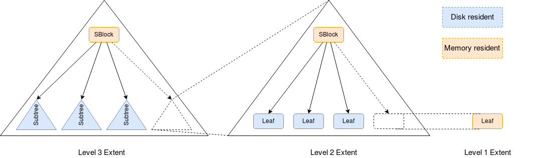
The picture shows B+trees with three extents and a fan-out ratio of 4 but real B+tree used by Akumuli have a fan-out ratio of 32. Note that each B+tree can be incomplete only from the right.

Tree construction

The tree construction algorithm is simple:

• Write new values to the level-1 extent (memory resident leaf node);
• If level-1 extent is full - write it to disk and add reference to it to the level-2 extent;
• If level-2 extent is full - write its root node to disk and add reference to it to the level-3 extent;
• Etc.

On the picture above, when the level 1 extent will be full, the leaf node will be committed to disk and take its place in level 2 extent (showed by dash lines), this will make the level 2 extent full and cause it to be merged with level 3 extent (showed by dash lines as well). After that, the level 4 extent will be created and extents 1-3 will become empty.

This process is an equivalent of the SSTable merge in LSM-tree. The number of extents is expected to be small because each leaf node contains many values (it contains a variable number of values because of compression) and the fan-out ratio is 32. Let’s do some back of the envelope calculations! If leaf node can store about 1000 data points than level 2 extent will be able to store 32000 data points and level 3 will be able to store more than 10 million. Akumuli limits the number of extents in each tree by 10. This is more than enough because with 10 levels we can store a series with more than 10^16 data points, e.g this is enough to store more than 300 years of data with microsecond precision.

Here come the advantages of the NB+tree over the LSM-tree:

• Memory resident part of the tree is small (single leaf node + several inner nodes);
• Many trees can live in one file and blocks of different trees can be interleaved on the storage level;
• Merge is very efficient. It’s enough to just add an address of the root node of the one extent to the other extent; no need to read the data and merge anything.
• We can store some information inside inner nodes to speed up aggregation and resampling of the time-series without maintaining some external data-structures (rollups) or indexes.
• Parallel operation. It is possible to write to the database from many writer threads (and Akumuli is doing this).
• Good for modern SSDs. All writes are aligned and performed in parallel. All tree nodes have the same size.

This data-structure allows Akumuli to maintain separate NB+tree instance for every time-series in the database. The primary disadvantage of this design is the complexity of the crash recovery process. It’s impossible to maintain WAL or command log per NB+tree instance. Akumuli uses a different approach to crash recovery that’s not discussed in this article but you can find more details about it in this article.

Ability to build separate NB+tree instance for every time-series is truly important. It enables queries in column-oriented fashion and, at the same time, it enables really fast parallel writes with very small write amplification. My recent experiment showed that it can write about 16 million data points per second on a c3.8xlarge instance.

Update

Hacker News discussion.