It’s been a while since Scylla team demonstrated that their highly capable database can read 1B (1.000.000.000) rows per second on an 83-node cluster. This is roughly 12M rows per second per server.

The task was simple: store temperature measurements from one million homes for one year with one-minute readings. That about a half of a trillion data points - 1.000.000 * 60 * 24 * 365 = 525.600.000.000 rows! Moreover, as if the sheer volume was not enough they introduced an outlier to the dataset. The outlier is a single reading that’s supposed to be found by the query. This setup was meant to show how well their consistent hashing works.

It didn’t end there though. Folks from Altinity decided to repeat the test with Clickhouse using Intel NUC as their server! The NUC despite being a tiny PC with inadequate cooling was outfitted with 4-core Intel i7 CPU, 32G of RAM, and most importantly 1Tb NVMe SSD. Clickhouse was able to load that dataset in 17 hours and find the ‘needle’ in 8.6 seconds (using the pre-built index). Their compression algorithm was able to trim every data point to just 1.6 bytes on average. This benchmark is interesting because it demonstrates that with the right software you can outmaneuver a big expensive setup using cheap commodity hardware. Kudos to the Altinity team!

I decided to build own version of the test. I don’t have an Intel NUC so I ended up using 12 vCPU ‘Standard’ DigitalOcean droplet (which is DO’s word for VM) because it’s the cheapest option that offers 1TB of SSD storage. This instance has 12 shared vCPUs which means three things. First, the CPUs are shared between different VMs on the same host so you can expect inconsistent performance. The CPUs are hyper threads, not real CPUs. Third, this setup is nowhere near as good as the real dedicated machine so it’s cheap! My goal was to spend less than $50 on hosting while doing this test to demonstrate that Akumuli is cost-effective.

Input Data

I wrote a script that generates the test data. I wanted to use 8 vCPU ‘Standard’ droplet to run the script and to load the data into Akumuli. This droplet has 640GB of storage. I had to tweak the input to fit this droplet. It still has 525.6B unique data-points and 1M homes but everything was divided evenly between 10 metrics (‘temp0’ - ‘temp9’). It allowed to batch up to 10 values together in the input file and as result ‘gzip’ was able to compress everything way better.

The data was generated using a random walk within reasonable bounds for temperature (19C to 35C). Instead of introducing a single outlier the script introduced a series of outliers. It selected 100 homes and for each of them, it generated a series that was growing randomly up to 100C.

It took around two days to generate the input files. The script that does this is called ‘gen.sh’. The output was around 200GB compressed and around 4TB uncompressed.

Loading the Data

Because I used the shared VM I repeated the experiment several times. The best load time I’ve seen was 6 hours, the worst one - 7. The variance was because both VMs had shared vCPUs.

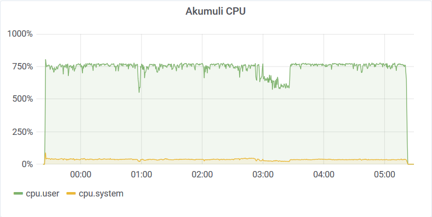
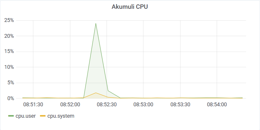
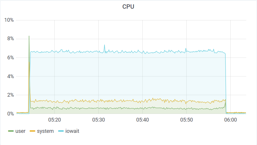
You can see that this run was affected by other VMs in the cloud by looking at this graph. I’ve been using 8 connections to load the data. This means that the Akumuli server could process the data using 8 threads. Akumuli doesn’t use all available CPUs for ingestion. It leaves some CPU power for queries so ingestion never makes the database unresponsive. On a 12 CPU machine, it uses only 8 CPUs for ingestion by default. The best-case ingestion speed was 24.319.822 elements / second. The network was quite busy too.

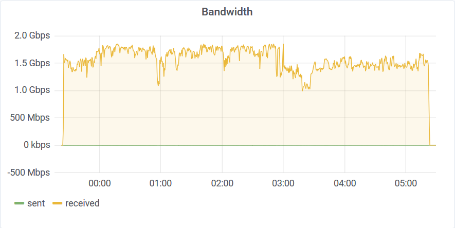
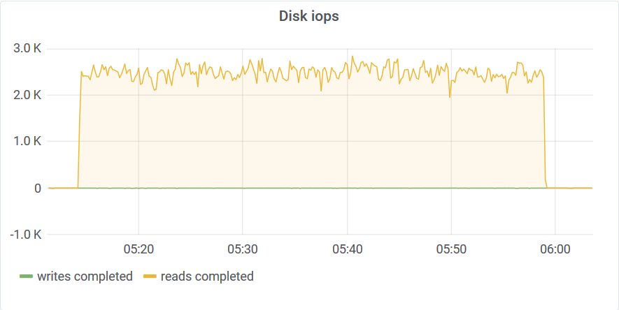
You can see that after 3 am something happened on the host machine. I never saw uneven distribution like this on dedicated hardware. The disk stats are also interesting:

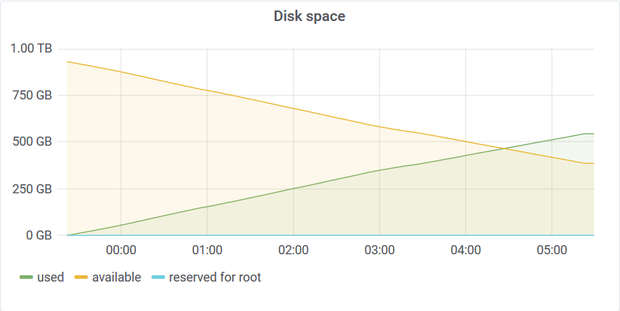
The disk usage at the end of the test was 554GB. This means that Akumuli used 1.1 bytes/reading on average. Akumuli uses a novel time-series compression algorithm which leverages next value prediction.

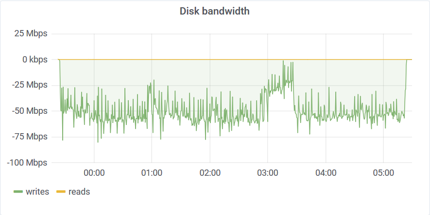
Curiously, you can see this 3 am dent on every graph. This graph tells us that akumulid was using just a tad above 50Mbps of disk bandwidth to sustain that 24M elements per second write rate. This is why we need good time-series compression in our lives!

Aggregate Queries

Akumuli can find a single ‘needle’ without much trouble because it supports aggregation on the storage level out of the box. The ‘aggregate’ query can give you the outlier and its timestamp but you have to run this query for every series. This query can run faster if the series was compacted. Because of that, I ran it for both compacted and not compacted storage.

Also, Akumuli runs every query in a single thread by design. To leverage parallelism you have to run several queries in parallel. Because of that, I have single aggregate queries that run in one thread using 10% of data, and parallel queries that run in ten threads using all data. All queries were performed on a full year time range.

Single Aggregate

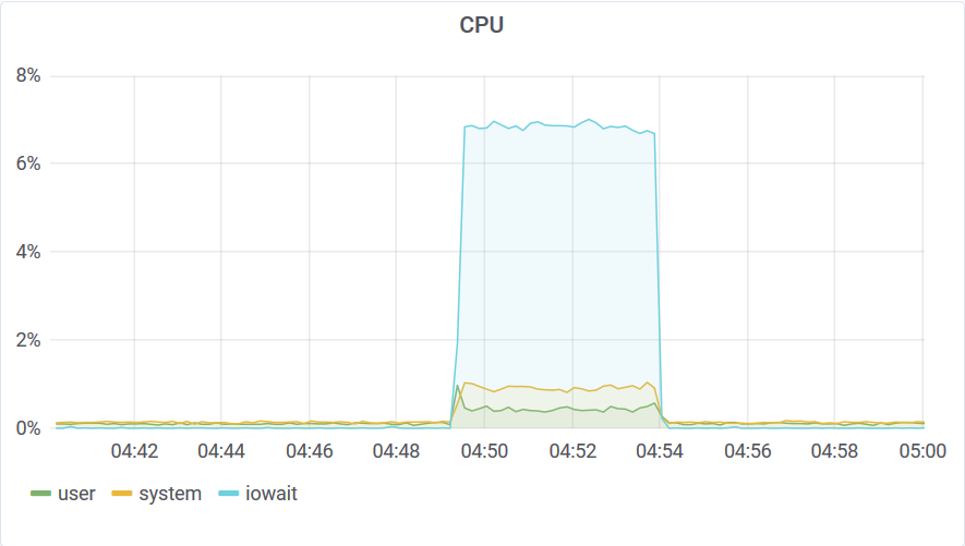
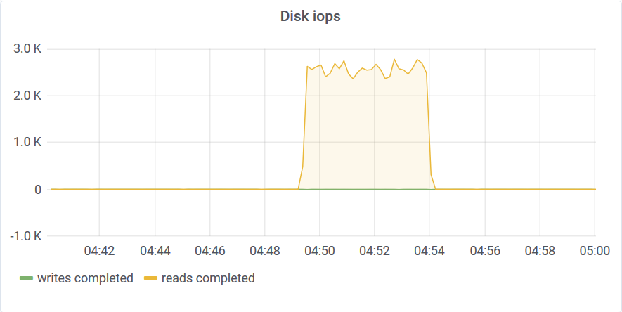
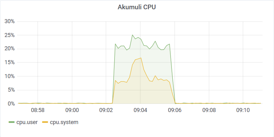
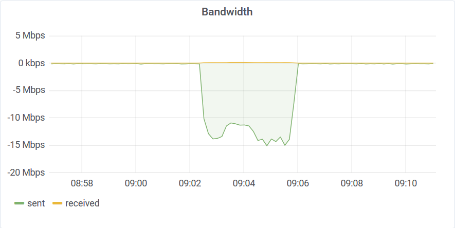
This query was performed on non-compacted storage. You can see that it took around 5 minutes to aggregate 52B data-points. This translates to a whooping 175M elements per second scan speed or 3ms execution time per series. Of cause it’s not a brute force scan.

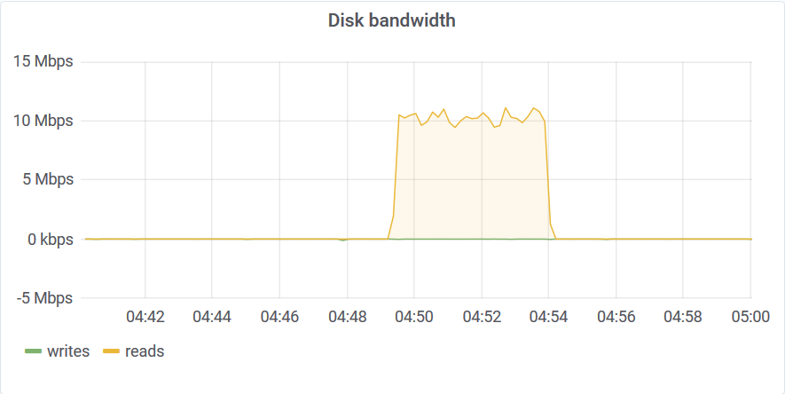
Only a small portion of the storage was scanned to compute the aggregates. You can read about the algorithm that makes this possible here. This query wasn’t limited by disk bandwidth or CPU speed but by the disk IOPS. This is a network-attached SSD and the IOPS throttled at around 3K.

Compacted Single Aggregate

If the storage is compacted aggregate query works faster. Long story short, it took 3 seconds to aggregate 52B data points.

Run aggregate query in one thread @ 20200303T085219
11305509        
                           
real    0m2.512s                                  
user    0m0.046s
sys     0m0.126s  
Completed @ 20200303T085222

The graph doesn’t have enough resolution to show that. Of cause, the reason for that performance is caching. Index nodes were compact and hot in the cache.

Parallel Aggregate

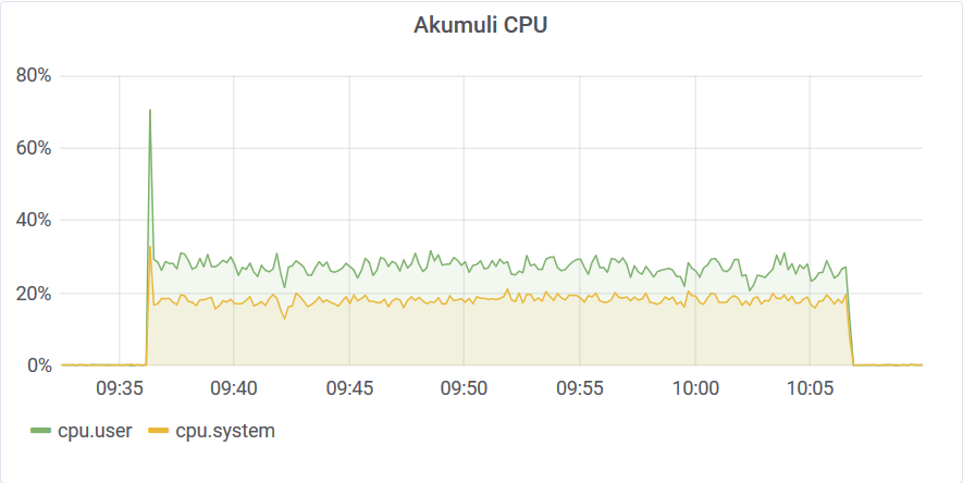
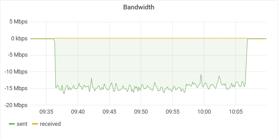
Let’s run the same query using 10 threads and 10 times more data!

You can see that it took around 45 minutes to aggregate 525B data points. This was because the query hit that 3K IOPS wall.

But it’s still good considering that we’re aggregated 1M series one by one wasting less than 3 ms per series.

Compacted Parallel Aggregate

On compacted storage, the same query was way faster since it needed to touch a smaller number of disk pages.

It took only 13 seconds to complete. The memory requirements for the query were quite moderate BTW.

You can see that the aggregate query does the job pretty quickly, but the downside is that it returns an outlier for every unique time-series. In our case, it returns 1M values which is a 100MB data transfer. This may not be what you want since your app has to parse all this data to find the top outlier among them. To get rid of this last step we can use a filter. The filter can be added to any other query (except aggregate) and it will filter out all data points that don’t match the filter requirements. Akumuli has some tricks under a sleeve to make this filter queries fast.

Single Filter

Let’s see how a single filter query performs. I’d set the threshold to 95C for this workload.

The query completed in 204 seconds. It streamed the outliers it found to the client.

Filter query doesn’t depend that much on compaction so there is no need to run it for both compacted and not compacted states.

Parallel Filter

Let’s try the same approach using 10 queries.

The filter query found every temperature reading above 95C in 30 minutes. The database transferred back around 3GB of data at 15Mbps.

The bottleneck here was once again a 3000 IOPS limit. This workload can run up to 10 times faster on dedicated hardware with normal SSD (tens of thousands IOPS) or up to 100 times faster on NVMe SSD (hundreds of thousand IOPS).

Conclusion

This benchmark wasn’t meant to represent real-world performance. Most likely you won’t be running queries like these and you won’t be loading the data the same way I did. If you want to benchmark Akumuli more realistically, try the TSBS benchmark suite. It supports Akumuli now.

Nevertheless, this shows what the database can do. Also, note that typical monitoring workloads don’t require the database to run such high-cardinality queries. And if you will run queries used in this test on single series you’ll often end up with sub-millisecond latencies. Also, note that Akumuli was never optimized for heavy queries that end up scanning the entire dataset. Given that, this is a great result. You can indeed load a huge dataset and analyze it. And most importantly, you can build interactive applications (e.g. monitoring dashboards) without much trouble.