NOTE: this article is out of date. Akumuli doesn’t work this way anymore.

Let’s talk about storage organization in akumuli. Time series data can be difficult to store. It is often generated during long periods of time and can be huge. This gives us two first requirements: compression and crash recovery. The significance of compression is obvious (let’s talk about it later). Crash recovery is a must if we don’t want to loose all data when somebody kills the app using the kill -9 command or if the app is killed due to—say—power outage. Databases are usually implemented in ways that prevent major data loss in such situations. They write new data to the write ahead log (WAL) first, fsync and only after that data can be written to the main storage.

Akumuli uses a different approach. All data is stored in one large WAL that consists from many volumes. Each volume is allocated beforehand and has a fixed size (4Gb). WALs are append-only. One can append new values or erase a volume entirely (this happens regularly to clean up some space for new data). What makes akumuli special is that there is no main data store. The WAL itself is the main data store and can be queried!

Volume structure

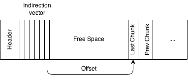
Each volume starts with a header. This header contains different useful kinds of information like volume size, number of data chunks stored, min and max timestamp inside volume and so on. One of the most important pieces of information in the header is an offset of the most recent data chunk.

The header is followed by the indirection vector. The indirection vector is an array of the offsets of the data chunks. This array is variably sized. When a new chunk is written to the volume its offset gets appended to the indirection vector. The offset of every chunk is stored in the indirection vector for quick access. Variably sized data chunks can be quickly fetched in random order using the volume’s indirection vector.

Each data chunk contains compressed time-series data from some time-range. Time-ranges of the different data chunks didn’t overlap. Data chunks are appended to the volume in starting from the end. A volume is full when there is no space between the indirection vector and the last data chunk.

This scheme is similar to a B-tree node structure in real databases except that the volume is huge compared to a B-tree node. This scheme allows akumuli to write data really quickly. Tests show that data can be written to the akumuli with really high pace - more then 1M writes per second on the m3.xlarge instance (with max crash recovery level and something about 6M with relaxed crash recovery).

Crash recovery

Akumuli msyncs data after each write in a two-step process. First msync triggered after new chunk was appended to the volume and its offset was stored in the indirection vector. Second msync triggered after update of the crash recovery register. This register stores index of the newest data chunk. During start-up akumuli gets last chunk index from this crash recovery register. If a failure occured during the first or second flush (or in between) this register would contain index of the previous chunk. If everything is OK it would contain the index of the most recent data chunk.

This may sound like a very slow process (lots of msync calls), but it isn’t the case because all writes are sequential and msync operation can be performed by the OS really fast.

Write trick

Akumuli maps all volumes into its address space. This can cause slowdown during write if a volume already contains data. The operating system doesn’t know that we are trying to rewrite a mapped file. Because of that it reads data into memory first. This can cause a huge slowdown. To workaround this akumuli uses a neat trick: When a volume needs to be overwritten we truncate the file to zero size and then expand it back. After that the operating system will know that the file is empty and nothing needs to be read back.

In the next part of this article I will talk about data compression. Stay tuned.