Recent major Akumuli release added support for write-ahead logging. This is a huge milestone for several reasons.
- It enables durable writes. Every time-series has a separate write buffer that could be lost in case of crash. Originally, Akumuli was developed with high-frequency data in mind. In this case it’s more important to restart the database after the crash as soon as possible. But if every series is updated rarely write buffers would contain hours of monitoring data.
- Previously, Akumuli used to open for writing every time-series in the database. Even the ones that wasn’t updated. With new WAL individual time-series could be opened for writing only when needed and also closed when they no longer needed. This helps to deal with situation when new series are created on the fly and the cardinality grows but only a subset of series are being updated.
- In the future it will allow to implement data replication via log shipping.
- Also, it will allow to implement backfill. Akumuli have a means to write data to the past but the process can be efficient only if the data is batched and WAL provides the batching mechanism.
There are some cons though. The most important one is performance degradation. Akumuli in WAL mode have to do some extra job. Every data point have to be logged and WAL volumes have to be rotated from time to time. I don’t want to go into details to much (wait for the next post) but you should know that WAL have to be updated more frequently than main storage and the data in WAL is less compact.
I decided to measure the difference between Akumuli with and without WAL. Here is my test setup!
- Load generator is a standard DigitalOcean droplet with 6-cores, 16GB of RAM and 320GB of disk space.
- Target server runs on general purpose DigitalOcean droplet with 8-cores, 32GB of RAM and 100GB of disk space.
Both droplets have 6TB of transfer which is enough for the test.
Test Data
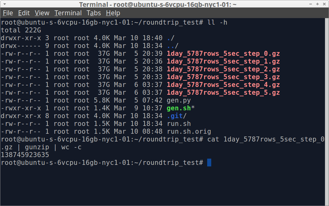
All benchmark code lives in this repository. To generate the data you have to clone it and run bash gen.sh. This script generates 6 gzip archives with test data in Akumuli format (the one that is normally used for ingestion). It takes many hours to finish and uses 222GB of disk space. This dataset should contain ~60-billion data-points from ~350000 unique time-series.
Individual series are generated using random walk algorithm. Every series name has six tags.
Target
On the target machine I installed Akumuli from the package repository. Then I configured it by running akumulid –init and editing ~/.akumulid configuration file. First of all I increased number of volumes to 20 (to use 80GB of disk out of available 100GB) and commented [WAL] section and all its elements. After that I created the database by running akumulid –create and started the server by running akumulid.
At this point I also setup the monitoring for both load generator and the target. I installed and configured Akumuli on load generator (all parameters left default). Also, I installed netdata on both machines. Both netdata instances was configured to send metrics in OpenTSDB format to the second Akumuli instance on load generator box. I also used apps plugin to generate metrics for the akumulid process. Also, I set up Grafana and installed Akumuli datasource plugin.
Running The Tests
To run the test ssh to the load generator and run bash run.sh. This script does two things. First of all it send data from every generated file to the Akumuli instance on the target machine in parallel. This is why 6-core droplet is needed. The data is sent via a bash itself using this syntax:
cat test-file.gz | gunzip > /dev/tcp/$IP/8282 &
Note that this command send uncompressed data so the actual transferred volume was not 222GB but close to 775GB. The second thing script does happens when all data is sent. It queries Akumuli instance on the target machine trying to fetch last data-point it had sent. It’s needed to make sure that all input was processed by the database server.
When run.sh finished I recorded the results, reconfigured target machine by resetting the database via
akumulid --delete
akumulid --create
and uncommenting the [WAL] section in the configuration file. After that I started akumulid on the target machine and run.sh on load generator.
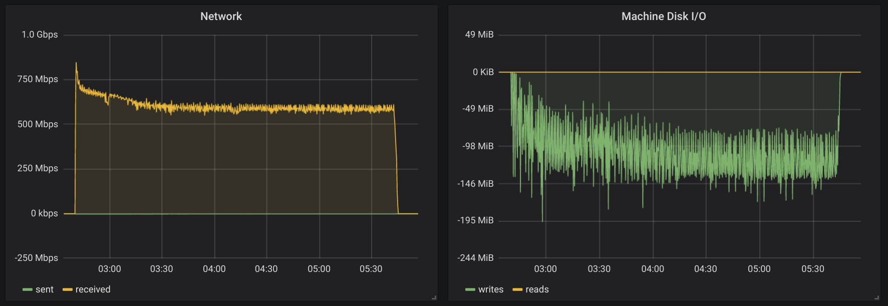
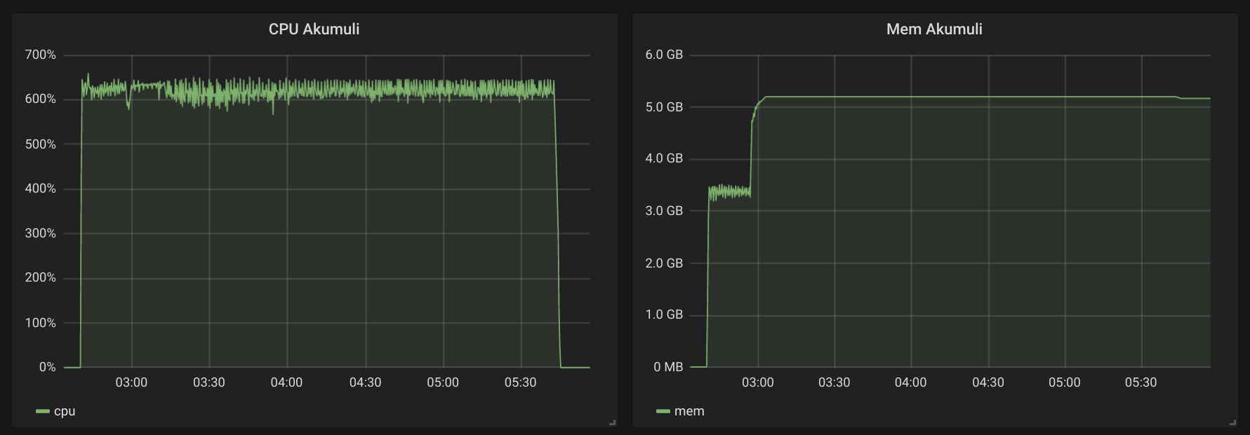
Here is how the first run looked like.
And here is the second one (with WAL).
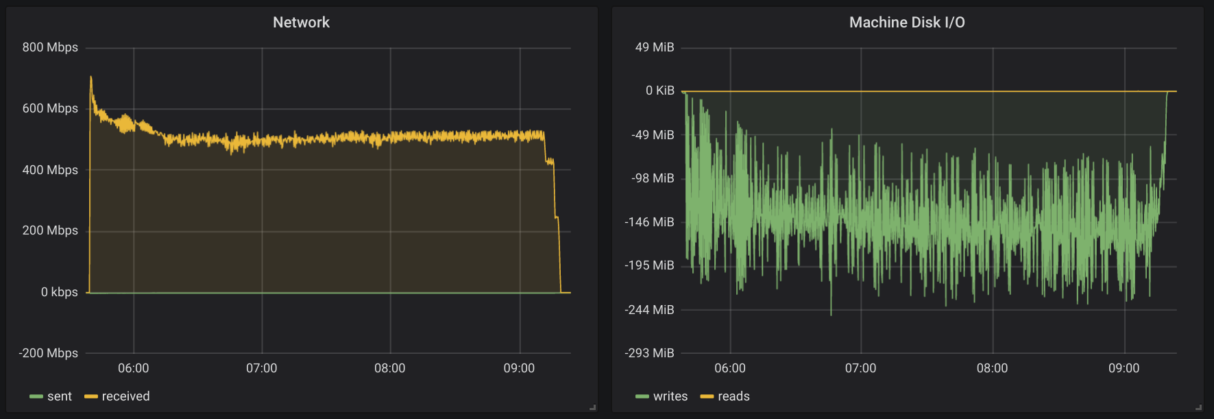
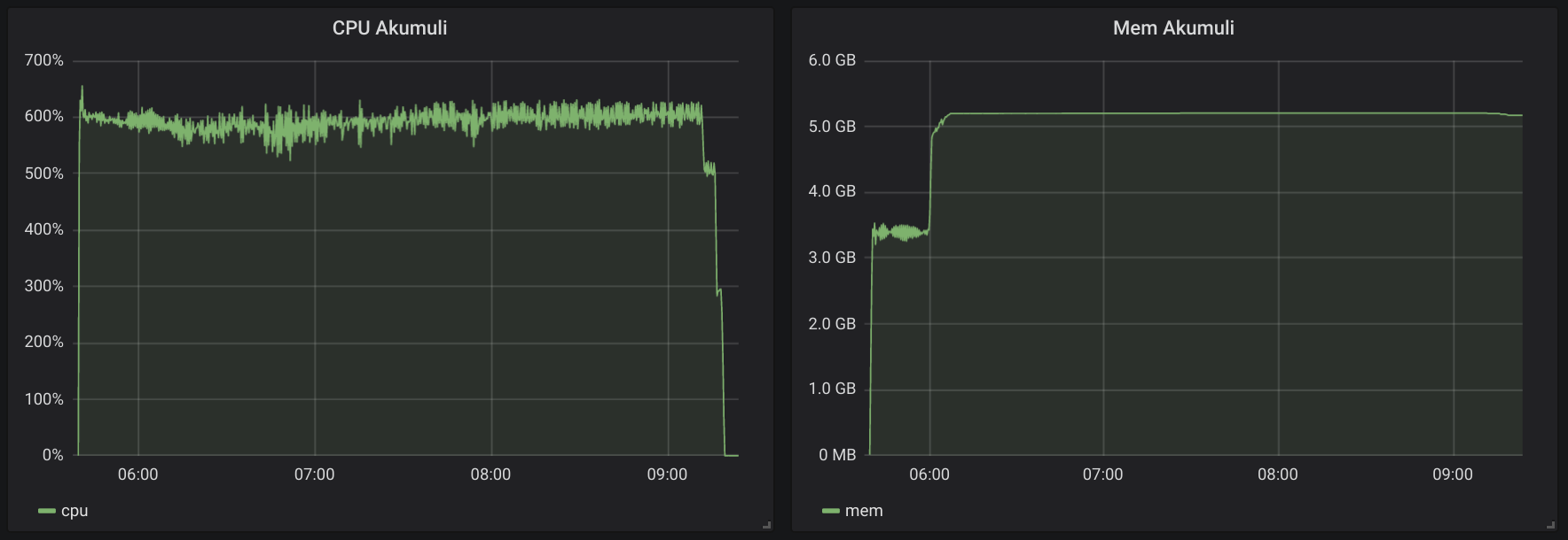
You can see that all graphs are somewhat close. Test duration was tad longer in the second run. And the Disk I/O graph is the most interesting one. It clearly shows that second run was writing more data.
Result
| No WAL | WAL | |
|---|---|---|
| Duration | 11090 seconds (3:04:50) | 13160 seconds (3:39:20) |
| Write rate | 5.410.244 datapoints/sec | 4.559.241 datapoints/sec |
| Relative speed | 100% | 82% |
The results are very predictable. I had the same close to 20% slowdown on my laptop with WAL enabled. But considering the overall performance the impact is not that big. In software engineering, performance was always traded for variety of good things like security or durability. Given the fact that Akumuli scales with added CPU-cores almost linearly and that every CPU-core gives you extra +1M writes per second the choice could be easy.
On the other hand, WAL uses extra disk throughput. This means that with WAL Akumuli will wear SSD faster. Also, WAL significantly increases recovery time.