The point of using a specialized time-series database is to have an edge over conventional databases in time-series specific operations. Most often, TSDB’s are judged by their write speed. In my opinion, the read performance is as important if not the most. Moreover, not only plain reads but filtering, aggregation, and downsampling operations which are used in every monitoring dashboard or alerting system.

Many TSDB’s use rollup aggregation mechanism to enable fast data resampling and aggregation. It works the following way. The user needs to create a set of rollup aggregation rules in advance. For instance, for every time-series in the database, she may want to store raw data, average values with 5-minute step, and average values with 1-hour step. The database will update these 5-minute and 1-hour rollups periodically. The user may set different retention policies for different rollups.

The problem with this approach is that the user must know in advance, what rollups she will need. Regenerating rollups can be costly and in some circumstances, impossible. Different time-series will need different aggregation function. For instance, for latencies we may want to use max but for free disk-space min is more suitable. Another problem is that the user must use proper rollup table in queries. Otherwise, the query will turn into a full table scan.

Another often ignored problem is that not all aggregations are composable. For instance, if you have averages with the 5-minute step but you need averages with 1-hour step you can’t just use these first 5-minute averages to compute the result. You need to compute it from raw data or you will get an incorrect result.

The final downside is the cardinality growth. Most modern TSDB’s struggles with high cardinality datasets (the ones that have a lot of unique time-series).

Akumuli solves this problem by resampling/aggregating the data on the fly. It uses some tricks to make this fast.

Akumuli stores each time-series in a B+tree. B+trees has two types of nodes. The leaf nodes are used to store compressed time-series data. Leaf nodes have fixed size. Because of that, each leaf has different capacity that depends on randomness and precision of the actual data. The inner nodes are used to store the links to other nodes. Akumuli stores the set of aggregates (like min, max, and sum) along with child address. Each aggregate corresponds to the entire subtree. The storage engine can use these values to your advantage.

Aggregation

This aggregates can be leveraged for various TSDB specific computations. The most simple use case is a data aggregation. Suppose that we need to find the largest value inside the time interval.

In the simplest case, the interval will span a whole number of leaf nodes. We just need to find the root nodes of all subtrees over which the time interval spans. No matter how large the time-span is and how many data-points it contains. We will read just a handful of pages from disk and use them to compose the result.

In this example, the time interval spans over nodes 10, 11, 12, and 13. To calculate an aggregate for it we need to read the root node 1 and proceed to inner nodes 2 and 3. Both of which has the links to subtrees that have the data we need (subtree 5, 10, 11, and subtree 6, 12, 13). The algorithm can extract the aggregates from 2->5 link, and from 3->6 link. After that this aggregates can be combined into the final result.

In the more complex scenario, the interval will span a fractional number of leaf nodes. The beginning and the end of the interval will be located in the middle of the corresponding leaf nodes. But here we may use divide and conquer approach. We can split the task into three parts:

1. Read the first page that partially crosses the time-interval. This will read the actual leaf node from disk, decompress it and compute max for every data-point that sits inside the interval.
2. Compute the max for the subtrees that sits inside the interval entirely, as described above.
3. Read the last page that partially crosses the time-interval, as in 1).

After that, we can compute final result by composing three max values (we should just get the largest one).

For instance, let’s look at figure 2.

1. First, we need to read page 9 (by following the path 1->2->4) and find the max value.
2. After that, we need to compute the max value in pages 10..13 by using pages 2 and 3 (the same way as in the previous example).
3. And finally, we need to read page 14 (by following the 1->3->7 path) and find the max value.

Downsampling

First of all, ‘group-aggregate’ query in Akumuli is not supposed to outperform pre-computed rollups. It supposed to be used in conjunction with Grafana and similar interactive tools. Because of this, some assumptions have to be made. Let’s state that the user usually reads the same number of data points with varying step and interval. This makes perfect sense for Grafana. If the size of the graph doesn’t change Grahana will vary the step and time interval in such way the number of points will be about the same. For instance, if the interval is 30 minutes, the step will be 1 second, but if the interval is 3 hours the step will be increased to 6 seconds or so. In both cases, the database should return about the same number of points.

Let’s look at naive approach first. The naive algorithm scans the series and calculates the downsampled series. For small steps, it’s a pretty good algorithm. But when the step becomes larger the amount of I/O needed growth linearly.

The optimized version utilizes aggregation as a subroutine. For every step interval, we should compute an aggregate. It’s done using the algorithm described above. The only trick is that the step 3) of the first interval and step 1) of the next step are combined. This algorithm requires the same amount of I/O as naive algorithm if the step is small. But the amount of I/O operations wouldn’t grow linearly. It have an upper bound that depends on the number of extracted data-points.

Let’s perform some back of the envelope calculations. Let’s state that 1 block always has 1300 data points with 1-second step (around 3 bytes per data-point) and the query should return 400 data-points.

	1 sec	30 sec	5 min	30 min	1 hour	12 hour	1 day
Optimized	4KB	37KB	370KB	1.5MB	1.5MB	1.5MB	1.5MB
Naive	4KB	37KB	370KB	2.1MB	4.3MB	52MB	104MB

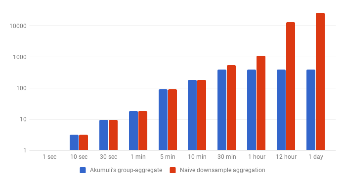
The naive approach will require the database to read around 37KB if the step is 30-seconds but if the step is 1-day the algorithm will read more than 100MB of data from disk. For the same query, the algorithm used by Akumuli will read only about 1.5MB. This is quite expensive compared to the rollup query. But on the other hand, it’s comparable with simple image download from a server.

Filtering

Akumuli also supports filter statement that can be added to select, join, and group-aggregate queries. This statement allows filtering time-series by value. This operation also utilizes pre-computed aggregates stored inside the B+tree nodes. The optimization is pretty simple. As the algorithm traverses the tree it may check does the link has any values that match the filter. If the subtree doesn’t have any it can be omitted. For instance, if we filtering out all values below 100 and the link to subtree has max=90 than we can safely prune the subtree from the search.

This approach works really well if we need to filter out everything but outliers. For instance, if no data point matches the filter the query will touch only root node of the tree. If all data points that match the filter are located in one leaf-node, the query will load only a couple of nodes. It will start from the root node and will follow the path until it reaches the leaf-node that has all the data we need.

Conslusions

These optimizations make a huge difference for many types of queries. An aggregate query execution lies within a millisecond range no matter the dataset. This means that it can be used as a subroutine in more complex algorithms. The filter query performance depends only on the number of returned data-points and works really fast if you need to search for outliers. And the downsampling aggregation can finally be used in interactive applications without any prior knowledge about the data and configuration.