In the previous article I discussed timestamps compression, now it’s time to talk about floating point data compression. This problem is not new, there are some good papers about it, e.g. Gorilla paper, and also this, and this one too. None of them is a good fit for Akumuli because the algorithms described in these papers are too specialized. The paper authors usually have a very specific dataset in mind. For example, Gorilla is optimized for slowly changed time-series and for integer time-series, and FCM algorithm will work best for scientific data.

So, I had to come up with a new algorithm. Simple delta encoding wouldn’t work at all. If you subtract one floating point number from the other, you won’t end up with the number that can be represented using a smaller number of bits. The solution here is to use bitwise XOR and get a binary diff instead of arithmetic delta.

Let’s get a closer look at IEEE 754 double-precision floating point number representation:

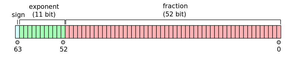
Fractional part occupies low 52 bits and sign and mantissa are located in high 12 bits. This means that if two numbers have close absolute values their high bits will be the same so when we XOR this values together, we will get a lot of leading zeroes in the result. Example: binary representation of 1.0 is 3ff0 0000 0000 0000 and binary representation of 1.0000000000000004 is 3ff0 0000 0000 0002. We will get 0000 0000 0000 0002 by XOR-ing this two values. This value occupies only two bits.

But some numbers will have very small (if any) number of leading zeroes when XOR-ed. E.g. 1.0 is represented as 3ff0 0000 0000 0000 and 2.0 is 4000 0000 0000 0000. By XOR-ing this two numbers we will get this result 7ff0 0000 0000 0000. This happens a lot in practice because many sources generate integers (e.g. number of bytes process is using, number of packets sent by the peer, etc).

So, we need to XOR not any but close values together. To achieve this Akumuli uses predictive coding. The idea is that we can try to predict next value and XOR it with the actual one. Basically, we will store prediction error. The predictor can be stateful, it can store some context information about the predicted signal. The signal usually is not totally random but stationary thus it can be predicted with some accuracy.

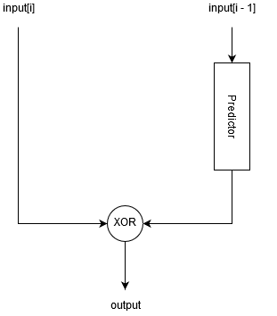
If our predictor is good prediction error will be small and we will be able to store it using a small number of bits. But what predictors should be used?

I’ve evaluated three predictors:

• Last value predictor.
• Finite Context Method (FCM) predictor.
• Differential FCM predictor.

(Actually, I’ve evaluated compositions of different predictors, but this is too much for the blog post)

Last value predictor (or delta modulator) assumes that the next value will be the same as the previous one. So, to use this predictor we can just XOR adjacent values of the array and we’re done.

FCM predictor is more complex. It predicts next value based on a finite number of preceding values. FCM predictor contains fixed sized table. This table maps contexts to values that were observed after particular contexts. The data structure is very simple:

struct FCM {
  double table[TABLE_SIZE];
  int last_hash = 0;
};

The update procedure should be used to add new values to the table:

double predict_next(FCM* fcm) {
  return fcm->table[fcm->last_hash];
}  

To understand how it works we should know how these values are calculated:

void update(FCM* fcm, double value) {
  fcm->table[fcm->last_hash] = value;
  fcm->last_hash = hash(value) % TABLE_SIZE;
}

To understand how it works we can imagine how FCM predictor of size two will be dealing with this input sequence: [-1, 1, -1, 1, -1, 1].

Obviously, last value predictor will fail here. Let’s define the hash function first. We need to extract some context from each floating point number, for FCM predictor of size two we can use sign bit:

int hash(double value) 
  if (value < 0.0) return 1;
  return 0;
}

Now let’s look how predictor will do its job:

• FCM initialized, table == [0, 0], last_hash == 0;
• predict_next(fcm) returned 0;
• update(fcm, -1), table == [-1, 0], last_hash == 1;
• predict_next(fcm) returned 0;
• update_next(fcm, 1), table == [-1, 1], last_hash == 0;
• predict_next(fcm) returned -1;
• update_next(fcm, -1), table == [-1, 1], last_hash == 1;
• predict_next(fcm) returned 1;
• udpate_next(fcm, 1), table == [-1, 1], last_hash == 0;
• predict_next(fcm) returned -1;
• …

So, FCM predictor can learn simple patterns like that. Basically, it remembers that some context (hash value) preceded some value and then when it meets this context it assumes that the value will follow. All we need to do is to give it some memory and proper hash function. It will be able to predict more complex patterns using more memory.

Famous Gorilla paper uses the algorithm that can be seen as a special case of the FCM compression with the table of size one. We already know it as “last value predictor”.

In Akumuli I’m using this hash function:

(last_hash << 5) ^ (value >> 50)

It extracts the sign, exponent, and two mantissa bits out of floating point number and blends it with some bits from the previous hash value. Blending previous hash bits is very important because it makes context depend on several adjacent values, not only the last.

DFCM works almost the same as FCM, but it works with differences, not the actual values.

I created this script to evaluate different predictors in different situations. It runs different predictors on several classes of input. Some of this classes are:

• Random walk;
• Steady growth trend;
• Pattern;

Random walk

This class of input is very important because it mimics a stationary process. This is the most important and general case. DFCM certainly has some advantage here, not overwhelming but noticeable.

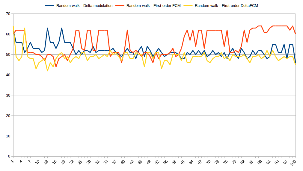
This graph shows number of bits needed to store each value using different predictors. X axis is a value index and Y axis is a number of bits needed to represent prediction error so, the smaller the value the better compression.

Pattern

Sometimes we need to represent the state of the system using discrete values (e.g. use 1 and 0 to represent on and off states). In many cases, this discrete values will form stable patterns because each value represents a state of some finite state machine and the state machine often goes through the same sequence of state transitions over and over again. Predictor should learn this patterns.

This is how three predictors compress repeating pattern composed of three discrete values:

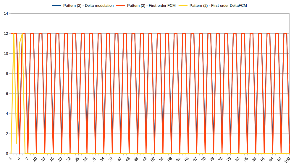
After just six iterations DFCM was able to predict the input perfectly. Both FCM and last value predictors performed poorly.

Steady growth trend

Some data sources are producing time-series with increasing values (e.g. number of packets sent, electricity consumption, etc). This is how our predictors performed on simple linear trend:

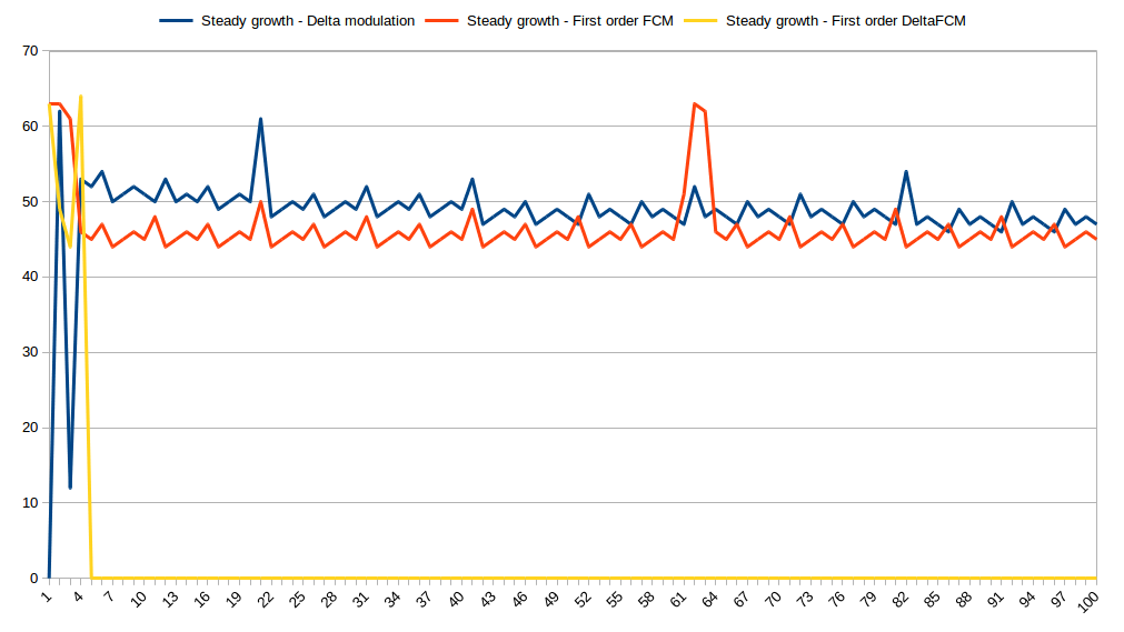
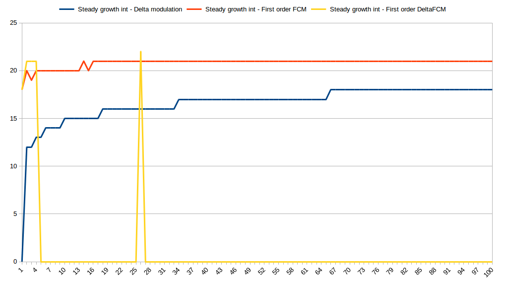
After several iterations, DFCM predictor started to predict input perfectly. Other two predictors couldn’t comply. We can see the same picture with integer time-series:

What if the trend will be random?

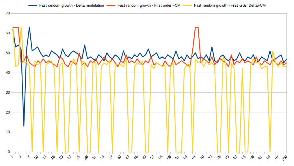
You can see that DFCM still outperforms other predictors but there are some spikes. We definitely will need more space to store this.

Final thoughts

As result of this evaluation, I’ve chosen DFCM predictor for Akumuli. It performs relatively good on monitoring data as well as scientific data. You can see that compression ratio depends on dataset heavily and predictive compression algorithm do make a difference in some cases. This article covers only small part of the algorithm, but you can check this design document for more details.